TELEMED Art Us RF Data Control II User Manual

 

Internet page: https://www.pcultrasound.com/

Information E-mail: info@pcultrasound.com

Support E-mail: support@pcultrasound.com

https://www.pcultrasound.com

 

Introduction

The document describes ArtUs RF Data Control II program from the release of the 2.1.4 version. The program is dedicated to the real-time acquisition of raw ultrasound data (channel RF data and beamformed RF) by using new unique configuration TELEMED scanner ArtUs. It’s a continuation of the predecessor just the structure of the interface controls was reorganized into tabs and new functionality to receive raw channel data in real-time and to control related acquisition parameters (active channels selection, transmit delays programming, programming of excitation pulses, etc.) was implemented.

By using the scanner and software equipped with channel data acquisition capabilities

you can:

1. To program custom transmit delay values for individual channels and apertures. Fully custom transmit focusing in terms of delays available.
2. To choose active channels from 64 available (trade-off between frame rate and image quality).
3. To program custom transmit pulses for all channels of electronics (Tri-state pulser +A, 0, -A).
4. To select arbitrary beams to scan (custom sequence of working apertures) from the available range of beams.
5. Analog front-end parameters will be available for the users (high-pass filter cut-off, input resistance, and gain).
6. Possibility to adjust custom analog depth-dependent amplification of received echoes.

You cannot:

1. To program different in terms of amplitude and shape excitation pulses (Tx), analog front-end parameters and analog amplification values and depths for individual channels of electronics.
2. Channel data supporting scanner operates only in B (brightness) mode, other modes like Doppler are not supported.

 

1. Structure of ArtUs RF Data Control II User Interface

Currently, ArtUs RF Data Control II program contains 6 tabs with different categories of ultrasonography controls:

• B controls
• RF controls
• Channel RF Data
• Data Recording
• Settings
• About

1.1. B Controls Tab and the other main components of GUI
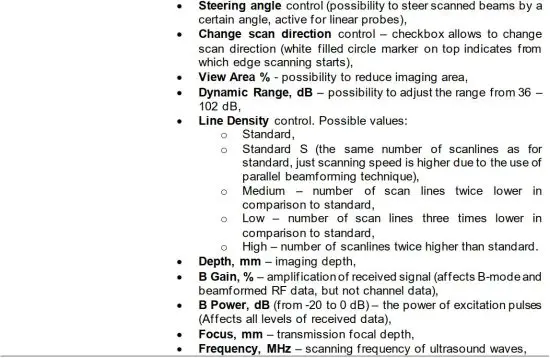
The subsection presents the B Controls Tab and other main components of GUI. The majority (all except post-processing algorithms which are applied on B-mode image) of B-mode imaging parameters available in the Echo Wave II application are also available for ArtUs RF Data Control II program.

 

 

1.2. RF Controls Tab
RF Controls Tab allows to 1) select from which point of the beamformer raw data will be received, 2) adjust the Size and Position of the RF window which defines the amount of RF data to be transferred and the relative position of the RF output window in the B-mode image frame.

 

1.3. Channel RF Data Tab
Channel RF Data Tab contains controls that affect raw channel data. The controls are divided into taking effect on 1) Transmit control and 2) Receive control of channels. NOTE: by entering into custom modes in Transmit control you can alter acoustic output values so you cannot use the device with biological organisms!!!! The screenshot of Channel RF Data controls is shown below:

 

 

Custom focusing delays – possibility to use custom transmit focusing by uploading *.txt file of transmit delays for individual channels. The structure of the *.txt files with the delays for different scanning cases are provided and possibilities are described in Appendix I. In the beginning, it is possible to store the delays used by implemented TELEMED scanning modes (B Standard, B Wide View and B Compound) by pressing the button Save to file… when the desired mode is selected in the B controls Tab. To load custom delays from the file button Upload file… must be used. For uploading custom transmit delays you must select Custom mode in the Combo box (Note! If Scan Type is changed and different *txt files are uploaded sequentially you must turn on Custom mode in the combo box again).

Arbitrary scanning beams – possibility to scan beams in arbitrary order (multiple repetitions of them etc.). Controlled by uploading *.txt file of beams indices to scan. The structure of the *.txt file with the example is provided and possibilities are described in Appendix II. For uploading the file you must select Custom mode in the Combo box.
The disappearing RF Window on the B-mode image is the indicator that custom mode is turned off for both delays and arbitrary beams since you are no longer scanning well-defined beams and channel RF data.

AGC control affects both B-mode images and channel RF data. The points can be created interactively by the left mouse click on the chart at the desired location and deleted by the right mouse click nearby point to delete. The points could be added by using edit fields (Depth, Value) and confirming by button Add (Insert button creates blank value). There is a possibility to Sort AGC points and Delete some points, to Copy, Paste, Save, and Load the AGC curve.
Note! AGC curve are connected with B Gain Control, Gain control shifts the programmed AGC curve down if decreased from 100 % linearly. 100 % gain means AGC as it is programmed, lower gain levels mean attenuated AGC by proportion to percent level.
3) AFE – analog front-end controls which effect on channel data could be controlled as well:

Note! For channel data mode ITHI frequency mode and Standard S line density options are not supported.

1.4. Data Recording Tab
ArtUs RF Data Control II software allows recording raw data into *.bin files. There are two different structures of the files: 1) channel data and 2) beamformed RF data. Channel data can only be recorded retrospectively when scanning is frozen from Cine Loop memory, meanwhile for beamformed RF Data it is possible to record RF Data in real-time, just such recording might result in a small number of missing frames and slightly reduced FPS. Data Recording Tab contains the following controls:

1.5. Settings Tab
Settings Tab allows to adjust Cine Loop size and to Save/Load used imaging settings into/from file, to choose probe if two ports Artus scanner is used

1.6. About Tab
About Tab discloses contact info of TELEMED manufacturer.

 

2. Recording of RF data files

Currently, ArtUs RF Data Control II software allows the recording of the RF data to binary files for channel mode and for beamformed RF data mode. There are two different structures of files for different types of RF data (channel RF and beamformed RF). Both structures have header information and RF data. The header contains some data acquisition parameters and information that is mandatory for B-mode image reconstruction from the recorded RF data.

2.1. Structure of the beamformed RF data file
The collected beamformed RF data and the main acquisition parameters needed for offline analysis and imaging could be recorded into binary files (*.bin). The filename contains acquisition time and date information, and the probe type code (HH.MM.SS_DD-MM-YYYY_probe_code.bin, i.e. “16.34.00_27-10-2017_L18-10H30-A4.bin”). The ArtUs RF Data Control SDK allows the recording of the RF data files of unlimited size (limited only by the capacity of the HDD).
Each recorded RF data frame contains header information and beamformed RF data from the corresponding RF window. The position and size of the window could be adjusted during scanning, and therefore the header of acquisition information is written to file for each frame in a recorded sequence. Please note that smaller window size allows to achieve higher frame rates. The file structure for a single frame is defined as follows:

 

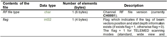
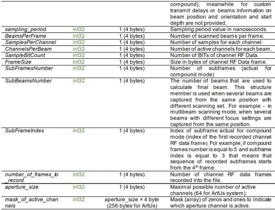
2.2. Structure of the channel data file
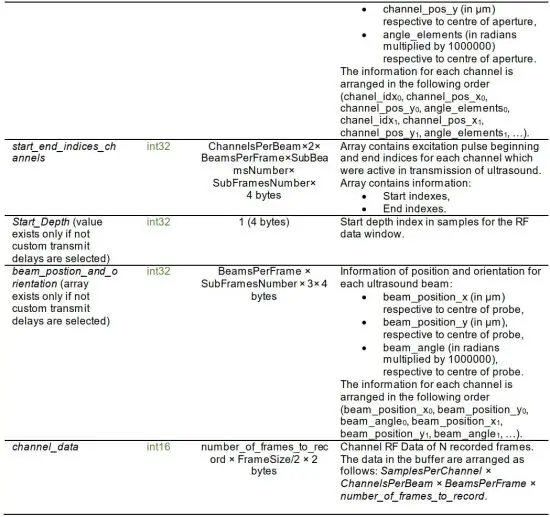
Channel data BIN file as beamformed RF data file contains header and channel data. The main difference is that header information is written only once before channel data frames and not before each channel data frame contrary to beamformed RF data files. The header contains information that is mandatory for B-mode image beamforming from channel data. Channel data could only be written after freezing scanning – retrospectively from Cine Loop memory to preserve data transfer speed. The file structure for channel data is defined as follows:

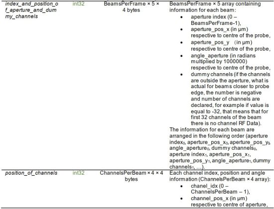
2.3. Coordinate system for B-mode image reconstruction
For channel data mode few arrays describe the position and orientation of beams (not always present), apertures, and channels, meanwhile for beamformed RF only the position and orientation of beam arrays are given. This subsection provides a drawing below how these coordinates are related (example for linear probe). Coordinates and angle (aperture_pos_x, aperture_pos_y, angle_aperture) of the aperture are physical meanwhile if the scanning beam was steered by a certain angle, you must use beam position and orientation arrays (beam_position_x, beam_position_y, beam_angle) for reconstruction. Please note the beam position and orientation information in the channel data file exists only if no custom transmit delays and beams are used during scanning. Both aperture coordinates and beam (if exist) coordinates are respective to the center of the probe (0,0). For each aperture/beam, there are provided channel position and orientation arrays (channel_pos_x, channel_pos_y, angle_elements) which provide information on how to position each channel in aperture. The drawing shows an aperture that contains 5 channels (elements) and probe center coordinates.

 

3. Installation notes and PC requirements

Requirements for the programming environment are as follows:

• To successfully run ArtUs RF Data Control II software the x64-bit Windows (8, 10, 11) operating system must be installed on your computer.
• i5/i7/i9 CPU
• 16 GB RAM or more
• USB 3.0
• Connected one of TELEMED ultrasound scanners:
  o ArtUs EXT-1H with RF module, beamformed RF data support
  o ArtUs EXT-2H with RF module, beamformed RF data support
  o ArtUs USS-1H, beamformed and channel RF data support
  o ArtUs USS-2H, beamformed and channel RF data support
• ArtUs properly installed drivers (for installation requirements please check the readme file of the drivers package).
• Installed Usgfw2 SDK x64-bit redistributable files (usgfwsetup.exe).

 

4. Revision History

 

5. References

[1] ArtUs RF Data Control User Manual.

 

Appendix I. Transmit delays file structure

There are 3 scanning modes for obtaining B image implemented in TELEMED ArtUs RF Data Control II software: 1) B Standard, 2) B Wide View, and 3) B Compound. By turning on one of these modes, you will receive certain limitations for custom delays file uploading. For B Standard and B Compound modes, only the same set of custom delays for each scanned beam could be applied, but for B Wide View mode you can program custom delays for each beam individually.

The table below describes the structure of delays files used for custom transmit focusing.

 

B Standard scanning mode example
[TX_header] Scan Type=0
Aperture Size=64
SubBeams Number=1
Beams Number=1
SubFrames Number=1
[Frame.0.Beam.0.SubBeam.0] Element.0=0
Element.1=0
Element.2=0
Element.3=0
Element.4=0
Element.5=0

Element.6=0
Element.7=0
Element.8=0
Element.9=0
Element.10=0
Element.11=0
Element.12=0
Element.13=0
Element.14=0
Element.15=0
Element.16=0
Element.17=0
Element.18=0
Element.19=0
Element.20=0
Element.21=0
Element.22=0
Element.23=0
Element.24=0
Element.25=0
Element.26=792
Element.27=795
Element.28=797
Element.29=798
Element.30=799
Element.31=800
Element.32=800
Element.33=799
Element.34=798
Element.35=797
Element.36=795
Element.37=792

Element.38=0
Element.39=0
Element.40=0
Element.41=0
Element.42=0
Element.43=0
Element.44=0
Element.45=0
Element.46=0
Element.47=0
Element.48=0
Element.49=0
Element.50=0
Element.51=0
Element.52=0
Element.53=0
Element.54=0
Element.55=0
Element.56=0
Element.57=0
Element.58=0
Element.59=0
Element.60=0
Element.61=0
Element.62=0
Element.63=0

B Wide View scanning mode example
[TX_header] Scan Type=1
Aperture Size=64
SubBeams Number=1
Beams Number=192
SubFrames Number=1
[Frame.0.Beam.0.SubBeam.0] Element.0=0
Element.1=0
Element.2=0

Element.3=0
Element.4=0
Element.5=0
Element.6=0
Element.7=0
Element.8=0
Element.9=0
Element.10=0
Element.11=0
Element.12=0
Element.13=0
Element.14=0
Element.15=0
Element.16=0
Element.17=0
Element.18=0
Element.19=0
Element.20=0
Element.21=0
Element.22=0
Element.23=0
Element.24=0
Element.25=0
Element.26=645
Element.27=645
Element.28=645
Element.29=645
Element.30=645
Element.31=645
Element.32=956
Element.33=952
Element.34=947
Element.35=942
Element.36=937
Element.37=931
Element.38=0
Element.39=0
Element.40=0
Element.41=0
Element.42=0
Element.43=0
Element.44=0
Element.45=0
Element.46=0
Element.47=0
Element.48=0
Element.49=0
Element.50=0
Element.51=0
Element.52=0
Element.53=0
Element.54=0
Element.55=0
Element.56=0
Element.57=0
Element.58=0
Element.59=0
Element.60=0
Element.61=0
Element.62=0
Element.63=0
[Frame.0.Beam.1.SubBeam.0] Element.0=0
Element.1=0
Element.2=0

Element.3=0
Element.4=0
Element.5=0
Element.6=0
Element.7=0
Element.8=0

Element.9=0
Element.10=0
Element.11=0
Element.12=0
Element.13=0
Element.14=0
Element.15=0
Element.16=0
Element.17=0
Element.18=0
Element.19=0
Element.20=0
Element.21=0
Element.22=0
Element.23=0
Element.24=0
Element.25=0
Element.26=488
Element.27=488
Element.28=488
Element.29=488
Element.30=488
Element.31=802
Element.32=798
Element.33=794
Element.34=789
Element.35=784
Element.36=779
Element.37=773
Element.38=0
Element.39=0
Element.40=0
Element.41=0

Element.42=0
Element.43=0
Element.44=0
Element.45=0
Element.46=0
Element.47=0
Element.48=0
Element.49=0
Element.50=0
Element.51=0
Element.52=0
Element.53=0
Element.54=0
Element.55=0
Element.56=0
Element.57=0
Element.58=0
Element.59=0
Element.60=0
Element.61=0
Element.62=0
Element.63=0
[Frame.0.Beam.2.SubBeam.0] Element.0=0
Element.1=0
Element.2=0
Element.3=0
Element.4=0
…………………………….

B Compound scanning mode example
[TX_header] Scan Type=0
Aperture Size=64
SubBeams Number=1
Beams Number=1
SubFrames Number=5

[Frame.0.Beam.0.SubBeam.0]
Element.0=0
Element.1=0
Element.2=0
Element.3=0
Element.4=0
Element.5=0
Element.6=0
Element.7=0
Element.8=0
Element.9=0
Element.10=0
Element.11=0
Element.12=0
Element.13=0
Element.14=0
Element.15=0
Element.16=0
Element.17=0
Element.18=0
Element.19=0
Element.20=0
Element.21=0
Element.22=0
Element.23=0
Element.24=0
Element.25=0
Element.26=823
Element.27=820
Element.28=816
Element.29=812
Element.30=808
Element.31=803

Element.32=798
Element.33=792
Element.34=786
Element.35=779
Element.36=772
Element.37=764
Element.38=0
Element.39=0
Element.40=0
Element.41=0
Element.42=0
Element.43=0
Element.44=0
Element.45=0
Element.46=0
Element.47=0
Element.48=0
Element.49=0
Element.50=0
Element.51=0
Element.52=0
Element.53=0
Element.54=0
Element.55=0
Element.56=0
Element.57=0
Element.58=0
Element.59=0
Element.60=0
Element.61=0
Element.62=0
Element.63=0

[Frame.1.Beam.0.SubBeam.0] Element.0=0
Element.1=0
Element.2=0
Element.3=0
Element.4=0

Element.5=0
Element.6=0
Element.7=0
Element.8=0
Element.9=0
Element.10=0
Element.11=0
Element.12=0
Element.13=0
Element.14=0
Element.15=0
Element.16=0
Element.17=0
Element.18=0
Element.19=0
Element.20=0
Element.21=0
Element.22=0
Element.23=0
Element.24=0
Element.25=0
Element.26=808
Element.27=808
Element.28=807
Element.29=806
Element.30=804
Element.31=802
Element.32=799
Element.33=796
Element.34=792
Element.35=788
Element.36=783

Element.37=778
Element.38=0
Element.39=0
Element.40=0
Element.41=0
Element.42=0
Element.43=0
Element.44=0
Element.45=0
Element.46=0
Element.47=0
Element.48=0
Element.49=0
Element.50=0
Element.51=0
Element.52=0
Element.53=0
Element.54=0
Element.55=0
Element.56=0
Element.57=0
Element.58=0
Element.59=0
Element.60=0
Element.61=0
Element.62=0
Element.63=0
[Frame.2.Beam.0.SubBeam.0] Element.0=0
Element.1=0
Element.2=0
Element.3=0
Element.4=0
Element.5=0

Element.6=0
Element.7=0
Element.8=0
Element.9=0
…………….

 

If some information in a *.txt file containing delay data is wrong you will receive an error message:

 

Appendix II. Arbitrary beams file structure
File structure for arbitrary beams is comparatively similar as in the case of transmit delays mode. The main two parameters are the count of beams (Beams Number) and the indices of beams to scan (Beams Indexes). The example below shows how to scan 5 beams with indexes 32, 96, 152, and 153. Indices correspond to certain spatial positions.

[Beams_header] Scan Type=0
Beams Number=5
[Beams Indexes] Beam.0=32
Beam.1=96
Beam.2=160
Beam.3=152
Beam.4=153

(c)1992-2024 TELEMED, UAB
——————————————————————————————-
Company address: Savanoriu pr. 178A, Vilnius, LT-03154, Lithuania
Internet: www.pcultrasound.com, www.telemed.lt
Information, sales e-mail: info@pcultrasound.com, info@telemed.lt
Technical Support e-mail: support@pcultrasound.com, support@telemed.lt

https://www.pcultrasound.com/

 

Read More About This Manual & Download PDF:

Documents / Resources

TELEMED Art Us RF Data Control II [pdf] User Manual Art Us RF Data Control II, RF Data Control II, Data Control II, Control II

References

• User Manual